Next: Mathematical description of a Up: Boundary conditions Previous: Multiple point constraints (MPC) Contents
In this section the theoretical background of the keyword *COUPLING followed by *KINEMATIC or *DISTRIBUTING is covered, and not the keyword DISTRIBUTING COUPLING.
Coupling constraints generally lead to nonlinear equations. In linear calculations (without the parameter NLGEOM on the *STEP card) these equations are linearized once and solved. In nonlinear calculations, iterations are performed in each of which the equations are linearized at the momentary solution point until convergence.
Coupling constraints apply to all nodes of a surface given by the user. In a kinematic coupling constraint by the user specified degrees of freedom in these nodes follow the rigid body motion about a reference point (also given by the user). In CalculiX the rigid body equations elaborated in section 3.5 of [19] are implemented. Since CalculiX does not have internal rotational degrees of freedom, the translational degrees of freedom of an extra node (rotational node) are used for that purpose, cf. *RIGID BODY. Therefore, in the case of kinematic coupling the following equations are set up:
This applies if no ORIENTATION was used on the *COUPLING card, i.e. the specified degrees of freedom apply to the global coordinate system. If an ORIENTATION parameter is used, the degrees of freedom apply in a local system. Then, the nodes belonging to the surface at stake (let us give them the numbers 1,2,3...) are duplicated (let us call these d1,d2,d3.....) and the following equations are set up:
The approach for distributing coupling is completely different. Here, the purpose is to redistribute forces and moments defined in a reference node across all nodes belonging to a facial surface define on a *COUPLING card. No kinematic equations coupling the degrees of freedom of the reference node to the ones in the coupling surface are generated. Rather, a system of point loads equivalent to the forces and moments in the reference node is applied in the nodes of the coupling surface.
To this end the center of gravity
![]() of the coupling surface is determined by:
of the coupling surface is determined by:
| (166) |
where
![]() are the locations of the nodes belonging to the
coupling surface and
are the locations of the nodes belonging to the
coupling surface and ![]() are weights taking the area into account for which
each of the nodes is “responsible”. We have:
are weights taking the area into account for which
each of the nodes is “responsible”. We have:
| (167) |
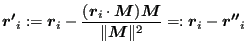
The relative position
![]() of the nodes is expressed by:
of the nodes is expressed by:
| (168) |
and consequently:
| (169) |
The forces and moments
![]() defined by the
user in the reference node
defined by the
user in the reference node
![]() can be
transferred into an equivalent system consisting of the force
can be
transferred into an equivalent system consisting of the force
![]() and the moment
and the moment
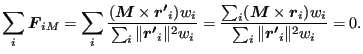
![]() in the center of gravity. Now, it can be shown by
use of the above relations that the system consisting of
in the center of gravity. Now, it can be shown by
use of the above relations that the system consisting of
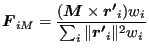
| (170) |
where
| (171) |
and
using the definition
 |
(173) |
is equivalent to the system
![]() in the center of
gravity. The vector
in the center of
gravity. The vector
![]() is the orthogonal projection of
is the orthogonal projection of
![]() on a
plane perpendicular to
on a
plane perpendicular to
![]() . Notice that
. Notice that
![]() and
and
![]() .
.
The proof is done by calculating
![]() and
and
![]() and
using the relationship
and
using the relationship
![]() . One obtains:
. One obtains:
| (174) |
| (175) |
 |
(176) |
 |
(177) |
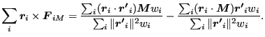
The last equation deserves some further analysis. The first term on the right
hand side amounts to
![]() since
since
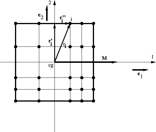
![]() . For the analysis of the second term a carthesian
coordinate system consisting of the unit vectors
. For the analysis of the second term a carthesian
coordinate system consisting of the unit vectors
![]() ,
,
![]() and
and
![]() is created
(cf. Figure 126 for a 2-D surface in the 1-2-plane). The
numerator of the second term amounts to:
is created
(cf. Figure 126 for a 2-D surface in the 1-2-plane). The
numerator of the second term amounts to:
| (178) |
These terms are zero (setting
![]() ) if
) if
![]() and
and
![]() i.e. if the carthesian coordinate system is parallel to the principal axes
of inertia based on the weights
i.e. if the carthesian coordinate system is parallel to the principal axes
of inertia based on the weights ![]() . Consequently, for Eq. (172) to be
valid,
. Consequently, for Eq. (172) to be
valid,
![]() ,
,
![]() and
and
![]() have to be aligned with the
principal axes of inertia! The equivalent force and moment
in the center of gravity are subsequently decomposed along these axes.
have to be aligned with the
principal axes of inertia! The equivalent force and moment
in the center of gravity are subsequently decomposed along these axes.
Defining
![]() and
and
![]() one can write:
one can write:
where
| (180) |
and
 |
(181) |
Notice that the formula for the moments is the discrete equivalent of the
well-known formulas
![]() for bending moments and
for bending moments and ![]() for torques
in beams [67].
for torques
in beams [67].
Now, an equivalent formulation to Equation (179) for the user
defined force
![]() and moment
and moment
![]() is sought.
In component notation Equation (179) runs:
is sought.
In component notation Equation (179) runs:
| (182) |
Defining vectors
![]() and
and
![]() such
that
such
that
![]() and
and
![]() this can be written as:
this can be written as:
| (183) |
or
| (184) |
where
![]() . This is a linear
function of
. This is a linear
function of
![]() and
and
![]() :
:
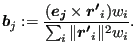
where
| (186) |
The coefficients
![]() and
and
![]() in
Equation (185)
are stored at
the beginning of the calculation for repeated use in the steps (the forces and
moments can change from step to step). Notice that the components of
in
Equation (185)
are stored at
the beginning of the calculation for repeated use in the steps (the forces and
moments can change from step to step). Notice that the components of
![]() and
and
![]() have to be calculated in the local
coupling surface coordinate system, whereas the result
have to be calculated in the local
coupling surface coordinate system, whereas the result
![]() applies in the
global carthesian system.
applies in the
global carthesian system.
If an orientation is defined on the *COUPLING card the force and moment contributions are first transferred into the global carthesian system before applying the above procedure. Right now, only carthesian local systems are allowed for distributing coupling.