Pipe, Gate Valve

Figure 117: Gatevalve

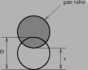
A gate valve (Figure 117) is characterized by head losses $\Delta_1^2 F$ of the form:

$$\Delta_1^2 F = \zeta \frac{\dot{m}^2}{2 g \rho^2 A^2 },$$ (158)

where $\zeta$ is a head loss coefficient depending on the ratio $\alpha=x/D$, $\dot{m}$ is the mass flow, g is the gravity acceleration and $\rho$ is the liquid density. $A$ is the cross section of the pipe, $x$ is a size for the remaining opening (Figure 117) and $D$ is the diameter of the pipe. Values for $\zeta$ can be found in file “liquidpipe.f”.

The following constants have to be specified on the line beneath the *FLUID SECTION, TYPE=PIPE GATE VALVE card:

• $A$
• $\alpha \;\;\;(0.125 \le \alpha \le 1)$

The gravity acceleration must be specified by a gravity type *DLOAD card defined for the elements at stake. The material characteristic $\rho$ can be defined by a *DENSITY card.

For the gate valve the inverse problem can be solved too. If the user defines a value for $\alpha \le 0$, $\alpha$ is being solved for. In that case the mass flow must be defined as boundary condition. Thus, the user can calculate the extent to which the valve must be closed to obtain a predefined mass flow. Test example pipe2.inp illustrates this feature.

Example files: pipe2, pipe, piperestrictor.